Creating a mesh from geometry using Gmsh

CHORAS uses Gmsh to create meshes. Gmsh provides a scripting language or serves as an API to geometry creation tools to define geometries and mesh them. This example assumes that the geometry has been defined and is provided in a Gmsh *.geo file.

For more information on Gmsh, please refer to the Gmsh documentation.

import numpy as np
import matplotlib.pyplot as plt
import gmsh
import matplotlib.tri as mtri

For Gmsh to work, it always needs to be initialized first.

gmsh.initialize()

Subsequently, the geometry file can be imported using the following function. Note that the function does not return anything, but the geometry is imported into the Gmsh model.

gmsh.open("example_room.geo")

Creating a surface mesh

Gmsh supports meshing in 1D, 2D, and 3D. For surfaces, a 2D mesh is appropriate. In Gmsh surface meshes can be accessed using

dim = 2

Different element types can be set using:

element_type = gmsh.model.mesh.getElementType("triangle", 1)

In Gmsh, different parts of the geometry can be grouped using Physical Groups. These can be used to identify different parts of the geometry and assign boundary conditions or material properties. The names of all surface groups can be accessed using:

surface_group_tags = gmsh.model.getPhysicalGroups(dim=dim)
surface_group_names = [
    gmsh.model.getPhysicalName(element_type, tag)
    for (element_type, tag) in surface_group_tags
]

To generate the surface mesh from the surface geometry, the following function can be used.

gmsh.model.mesh.generate(dim)

The Cartesian coordinates of all mesh nodes can be accessed using the following functions. All functions return the ids of the nodes as well as their coordinates as flat array. Accordingly, the coordinates need to be reshaped to a (N, 3) array for further processing.

node_tags_all, coords_all, _ = gmsh.model.mesh.getNodes()
coords = coords_all.reshape((len(node_tags_all), 3))

To access the nodes belonging to a specific surface group using their name, the following functions can be used to access the node ids for the triangular surface mesh elements. Note that the node ids start at 1 instead of python’s indexing which starts at 0.

mesh_kind = 3
dim_tags = gmsh.model.getEntitiesForPhysicalName(surface_group_names[0])
_, node_tags_group = dim_tags[0]

face_nodes = gmsh.model.mesh.getElementFaceNodes(
    dim, mesh_kind, tag=node_tags_group)
faces = np.reshape(face_nodes, (len(face_nodes) // mesh_kind, mesh_kind))

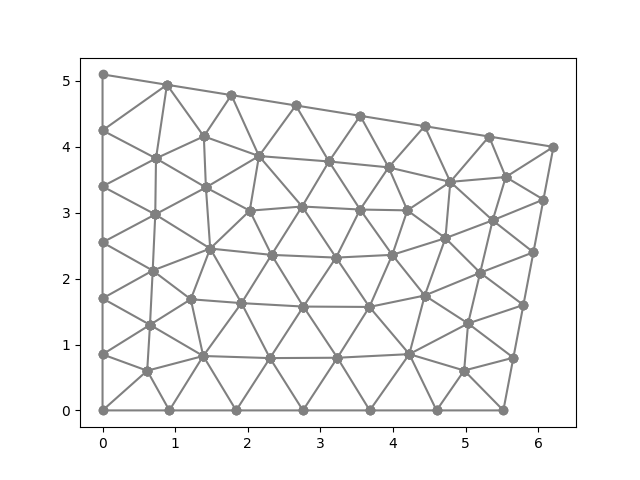
The mesh of the first surface group can be visualized using matplotlib. Note again that the node ids start at 1, hence the need to subtract 1 for numpy and matplotlib indexing.

tri_plotting = mtri.Triangulation(
    coords[:, 0],
    coords[:, 1],
    faces-1
)

ax = plt.axes()
ax.scatter(coords[faces-1, 0], coords[faces-1, 1], color="gray")
ax.triplot(tri_plotting, color="gray")
plt.show()

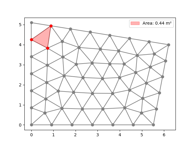
Calculating surface areas

The surface area of each triangular element can be calculated using the cross product of two sides of the triangle.

x = coords[faces-1][:, 0]
y = coords[faces-1][:, 1]
z = coords[faces-1][:, 2]
surface_areas = 0.5 * np.linalg.norm(
    np.cross(y - x, z - x, axis=-1),
    axis=-1)

surface_area_group = np.sum(surface_areas)
print(f"Surface area of {surface_group_names[0]}: {surface_area_group:.2f} m²")

Surface area of M_2: 26.88 m²

As an example, the first polygon of the surface group is highlighted in red and its area is shown in the legend.

ax = plt.axes()

idx_polygon = 0

ax.scatter(coords[faces-1, 0], coords[faces-1, 1], color="gray")
ax.triplot(tri_plotting, color="gray")
ax.scatter(
    coords[faces[idx_polygon]-1][:, 0],
    coords[faces[idx_polygon]-1][:, 1],
    color="red")
ax.fill(
    coords[faces[idx_polygon]-1][:, 0],
    coords[faces[idx_polygon]-1][:, 1],
    color="red", alpha=0.3, label=f"Area: {surface_areas[idx_polygon]:.2f} m²")
plt.legend()
plt.show()